1.2. Asymptotes

Définition

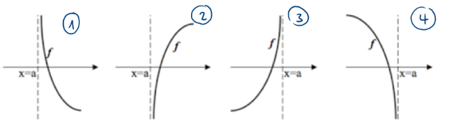
On dit qu'une droite verticale d'équation \(x = a\) est une asymptote verticale (A.V.) de la fonction \(f\) si l'une au moins des conditions suivantes est satisfaite :

\[\begin{array}{cccc} \lim_{x \to a^-} f(x) = -\infty & \lim_{x \to a^+} f(x) = +\infty & \lim_{x \to a^-} f(x) = +\infty & \lim_{x \to a^+} f(x) = -\infty \\ \text{(1)} & \text{(2)} & \text{(3)} & \text{(4)} \end{array}\]

Illustration

Exemple

Considérons la fonction réelle: \( f(x)=\frac{2}{x+3}.\)

Etapes:

I. \(D_f = \mathbb{R} \setminus \{-3\}\)

II. Intuitivement on pourrait donc penser que cette fonction a une asymptote verticale d’équation : \(x = -3\)

III. Vérification :

Conclusion : \( \text{f}\) admet une AV en \(x=-3\)

Remarques

1. « Si \( a \notin D_f \), alors \( f \) possède une asymptote verticale d’équation en \( x = a \). » Cette affirmation est fausse, car il se peut qu'une fonction possède une trou.

   Par exemple : \[ D_f = \mathbb{R} \setminus \{2\}, \quad f(x) = \begin{cases} 2x & \text{si } x < 2 \\ x^2 & \text{si } x> 2 \end{cases} \]

2. Le graphique d'une fonction ne coupe jamais une asymptote verticale.

   \[D_f = \mathbb{R} \setminus \{a\}\]

   Si une fonction admet une AV en \( x = a \) alors \( f \) est continue et \( f \in D_f \). Si un graphe coupe l'AV alors cela signifie qu'il existe une image en \( x = a \) ce qui est impossible.

§. 1.2.2 Les asymptotes horizontales

Définition :

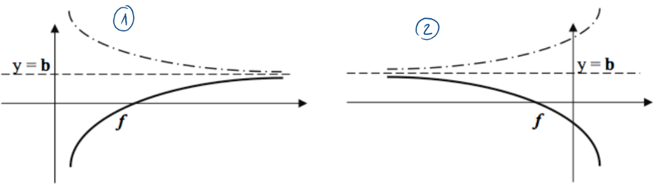
On dit qu'une droite horizontale d'équation \( y = b \) est une asymptote horizontale (A.H.) de la fonction \( f \) si l'une au moins des conditions suivantes est satisfaite :

\( \lim_{x \to +\infty} f(x) = b \) (1) ou \( \lim_{x \to -\infty} f(x) = b \) (2)

Illustration

Exemple

Soit la fonction réelle f définie par \(f(x) = \frac{4x + 3}{2x + 1}\)

Etapes :

I.\(D_f = \mathbb{R} \setminus \{-\frac{1}{2}\}\)

II. A.V. : en \(x = -\frac{1}{2}\) ?

\( \lim_{x \to -\frac{1}{2}^-} \frac{4x+3}{2x+1} = \frac{1}{0^-} = -\infty \)

\( \lim_{x \to -\frac{1}{2}^+} \frac{4x+3}{2x+1} = \frac{1}{0^+} = +\infty \)

III. A.H. : en \(y = 2\)

\( \lim_{x \to \pm\infty} \frac{4x+3}{2x+1} = \lim_{x \to \pm\infty} \frac{x \cdot (4 + \frac{3}{x})}{x \cdot (2 + \frac{1}{x})} = \frac{4}{2} = 2 \)

IV. Conclusion

• \(f\) admet une AV en \(x=-\frac{1}{2}\)

• \(f\) admet une AH \(x=2\)

Remarques

a) Dans les calculs, on peut encore préciser en cas d'A.H. si \(\lim_{x \to -\infty} f(x) = b^+\) , \(\lim_{x \to -\infty} f(x) = b^-\)

\(\lim_{x \to +\infty} f(x) = b^+\) ou \(\lim_{x \to +\infty} f(x) = b^-\). Cela peut aider s'il faut ensuite représenter

graphiquement \(f\).

b) Une fonction peut n'avoir aucune asymptote (comme les fonctions polynomiales), une seule (comme la fonction tangente, la fonction logarithme) ou plusieurs (comme les fonctions rationnelles, ...).

c) Le graphique d'une fonction peut, dans certains cas, couper une asymptote horizontale.

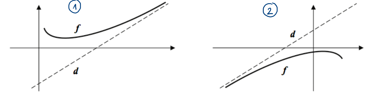
Définition :

Autrement dit, si \(x\) tend vers \(\pm \infty\), alors la différence entre \(f\) et \(d\) tend vers 0.

Illustrations

Exemple

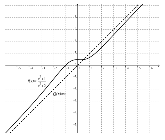
Soit la fonction rationnelle \( f(x) = \frac{x^3 + 1}{x^2 + 2} \text{ avec } D_f = \mathbb{R} \)

Effectuons la division euclidienne \(A(x)\) par \(B(x)\) :

\[ \begin{aligned} &\overbrace{x^3 + 1}^{A(x)} = \underbrace{x^2 + 2}_{B(x)} \cdot \overbrace{\color{red}{X}}^{Q(x)} + \underbrace{\color{green}{-2x + 1}}_{R(x)} \\[10pt] &(1) \Rightarrow x^3 + 1 = (x^2 + 2) \cdot \color{red}{X} + \color{green}{-2x + 1} \\ &\text{avec } \deg(R(x)) < \deg(B(x)) \\[10pt] &(2) \Rightarrow f(x)=\frac{x^3 + 1}{x^2 + 2}=\color{red}{X} + \frac{\color{green}{-2x + 1}}{x^2 + 2} \end{aligned} \]

L'asymptote oblique est donc donnée par la fonction \(Q(x)=x\)

Vérification :

\( \lim_{x \to \pm\infty} [f(x) - d(x)] = \lim_{x \to \pm\infty} \left[x + \frac{-2x+1}{x^2+2} - x\right] = \lim_{x \to \pm\infty} \frac{x \cdot (-2 + \frac{1}{x})}{x^2 \cdot (1 + \frac{2}{x^2})} \)

\(= \frac{-2}{\pm\infty} = 0\)

\(\Rightarrow y = x \text{ est l'AO de } f\)

Illustration

Remarques

a) Pour les fonctions rationnelles, il y a existence d'une asymptote oblique si le degré du numérateur = degré du dénominateur + 1.

Autrement dit : \( f(x) = \frac{A(x)}{B(x)} \) avec \( A(x) \) et \( B(x) \) des polynômes. Alors

\( \deg(A) = \deg(B) + 1 \)

b) Si \( a = 0 \) et \( b \neq \pm\infty \) de l'asymptote oblique, alors on a en fait une asymptote horizontale (d'équation y=b)

c) Une fonction ne peut pas avoir une A.H. et une A.O. du même «côté».

d) Le graphique d'une fonction peut dans certains cas couper une asymptote oblique.

e) Pour certaines fonctions (log, exp,...) il existe une A.H. ou A.O. en \(-\infty\) et une autre A.H. ou A.O. en \(+\infty\).